NV² | scripts for SocLab

scripts for SocLab

Presentation
Examples
Download
References

If you are using these scripts, please cite:

N. Villa-Vialaneix, C. Sibertin-Blanc and P. Roggero. Statistical exploratory analysis of agent-based simulations in a social context. Case Studies in Business, Industry and Government Statistics, 5(2), 132-149, 2014.

This project has been funded by the Maison des Sciences de l’Homme et de la Société de Toulouse (2012 grant, project SocLab-Stat).

Presentation

This page presents the R scripts developed during Soraya Popic’s insternship (March-June 2012) for analyzing a set of simulation outputs coming from the social simulation platform SocLab (see (El Gemayel et al., 2011) in the References section for the model description). More precisely, the scripts allow the user to:

make correlation analyses between pairs of variables: the correlations are displayed using an elliptical plot which is handy for interpretation;
project the data onto a 2-dimensional space with MDS (Multi-Dimensional Scaling) to help understand their dispersion and outline outliers;
make a clustering (Hierarchical Clustering) of the simulations to extract homogeneous groups of simulations and to explain according to variables in the dataset;
project the data onto a map using self-organizing map algorithm for combining clustering and visualization.

Examples

Using the dataset simulation-Seita.csv described in the Download section, the following results can be produced (for further details on the interpretation of these results, see the user reference manual in the Download section; other examples and references on the methods are also provided in this manual):

Pairwise correlation analysis

corMat <- CORR(delVar="ChefAtelier.SeuilSatisfaction,OuvProd.SeuilSatisfaction,
                       OuvEnt.SeuilSatisfaction",
               save=TRUE)
corMat

gives the following image:

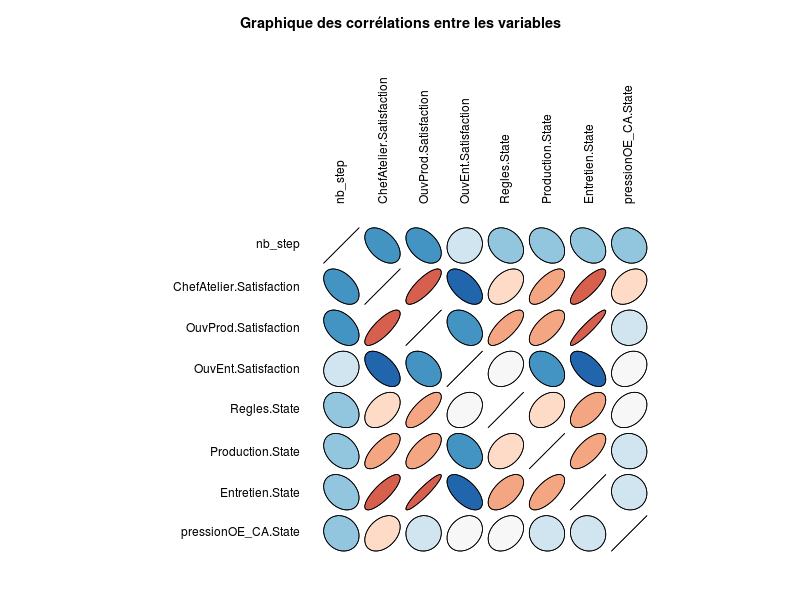
which is automatically saved into the directory from which the data file has been loaded. The corresponding table is also saved in the variable corMat:

                            nb_step ChefAtelier.Satisfaction
nb_step                   1.0000000               -0.4693084
ChefAtelier.Satisfaction -0.4693084                1.0000000
OuvProd.Satisfaction     -0.4315559                0.7967726
OuvEnt.Satisfaction       0.1008425               -0.5588591
Regles.State             -0.2690996                0.4387532
Production.State         -0.3171620                0.7047440
Entretien.State          -0.3204857                0.8116321
pressionOE_CA.State      -0.1375683                0.3689689
                         OuvProd.Satisfaction OuvEnt.Satisfaction Regles.State
nb_step                           -0.43155593           0.1008425   -0.2690996
ChefAtelier.Satisfaction           0.79677260          -0.5588591    0.4387532
OuvProd.Satisfaction               1.00000000          -0.3538305    0.7469297
OuvEnt.Satisfaction               -0.35383047           1.0000000    0.2868126
Regles.State                       0.74692966           0.2868126    1.0000000
Production.State                   0.65380700          -0.3560256    0.3594083
Entretien.State                    0.93097369          -0.5983080    0.5732658
pressionOE_CA.State                0.02304079           0.2527884    0.3056840
                         Production.State Entretien.State pressionOE_CA.State
nb_step                       -0.31716205     -0.32048568         -0.13756834
ChefAtelier.Satisfaction       0.70474399      0.81163209          0.36896887
OuvProd.Satisfaction           0.65380700      0.93097369          0.02304079
OuvEnt.Satisfaction           -0.35602556     -0.59830803          0.25278843
Regles.State                   0.35940826      0.57326577          0.30568404
Production.State               1.00000000      0.68088179         -0.02784973
Entretien.State                0.68088179      1.00000000         -0.05848475
pressionOE_CA.State           -0.02784973     -0.05848475          1.00000000

MDS and outlier detection with bagplot

mdsProj <- MDS(delVar="ChefAtelier.SeuilSatisfaction,OuvProd.SeuilSatisfaction,
                       OuvEnt.SeuilSatisfaction",
               bagPlot=TRUE,save=TRUE)
mdsProj$x
mdsProj$y

gives the following images:

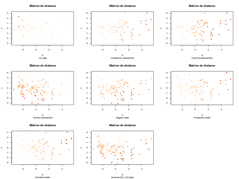
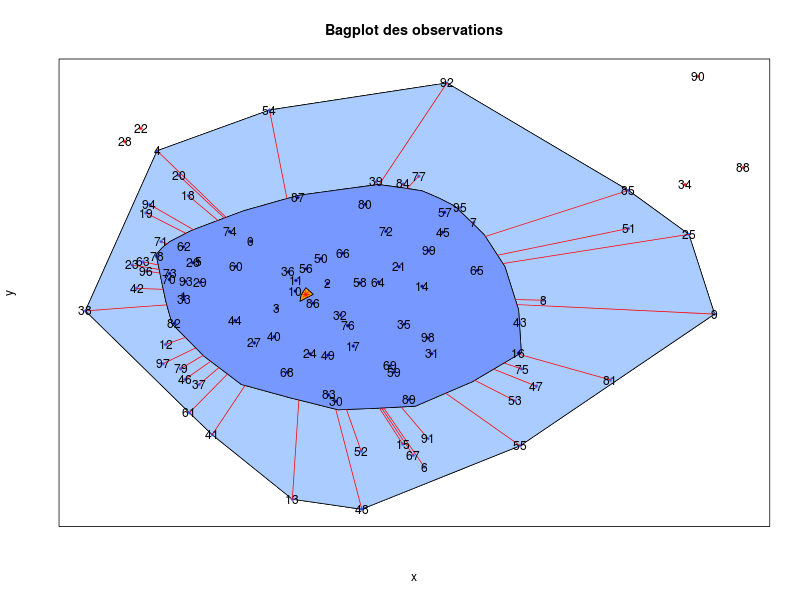
that are automatically saved into the directory from which the data file has been loaded. The coordinates of the simulations in the projection (respectively mdsProj$x and mdsProj$y) are also saved in the variable mdsProj.

Hierarchical clustering

classif <- CAH(manSelect=TRUE,delVar="ChefAtelier.SeuilSatisfaction,OuvProd.SeuilSatisfaction,
                                      OuvEnt.SeuilSatisfaction",
               MAV=TRUE,save=TRUE)
classif

gives the following images:

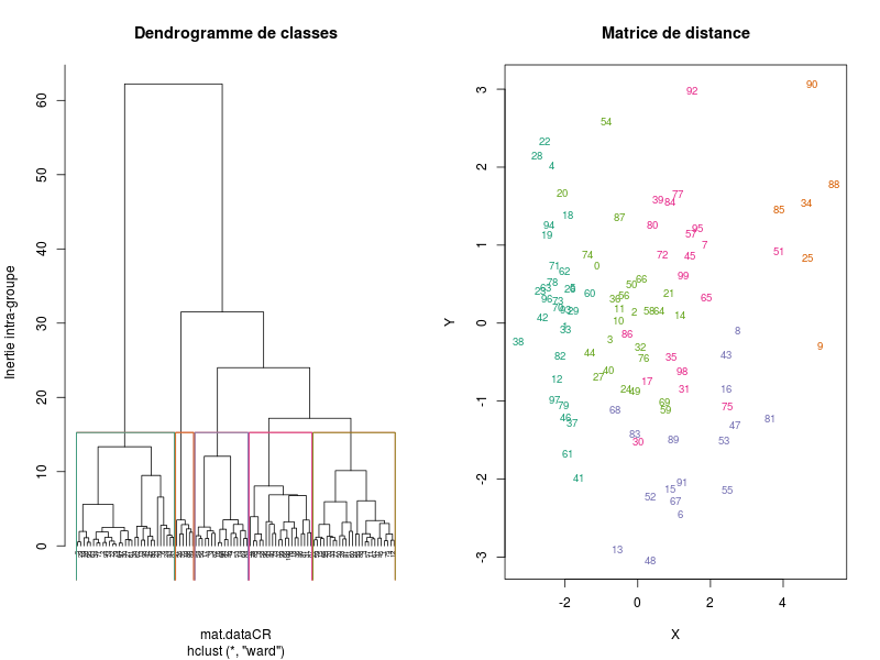
(on which the number of clusters can be chosen interactively, here the chosen number of clusters is 5)

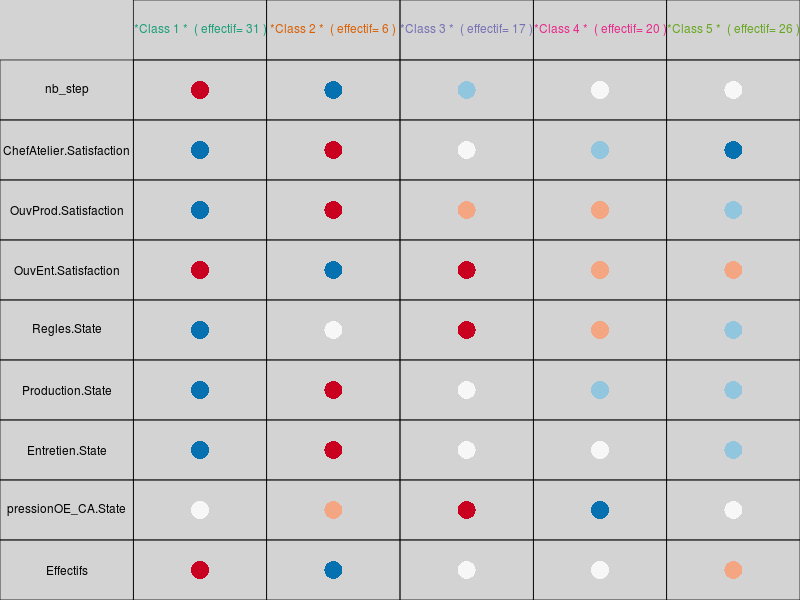
that are automatically saved into the directory from which the data file has been loaded. The table containing the variables averaged by clusters is also automatically saved in a file simulation-Seita-CAHanalyseMoy5Cl.csv. The cluster number for each simulation is saved in the variable classif:

  1   2   3   4   5   6   7   8   9  10  11  12  13  14  15  16  17  18  19  20 
  1   2   1   1   2   2   3   4   3   5   1   1   2   3   1   3   3   4   2   2 
 21  22  23  24  25  26  27  28  29  30  31  32  33  34  35  36  37  38  39  40 
  1   1   2   2   1   5   2   1   2   2   4   4   1   2   5   4   1   2   2   4 
 41  42  43  44  45  46  47  48  49  50  51  52  53  54  55  56  57  58  59  60 
  1   2   2   3   1   4   2   3   3   1   1   4   3   3   1   3   1   4   1   1 
 61  62  63  64  65  66  67  68  69  70  71  72  73  74  75  76  77  78  79  80 
  2   2   2   2   1   4   1   3   3   1   2   2   4   2   1   4   1   4   2   2 
 81  82  83  84  85  86  87  88  89  90  91  92  93  94  95  96  97  98  99 100 
  4   3   2   3   4   5   4   1   5   3   5   3   4   2   2   4   2   2   4   4

Self-Organizing Map

somRes <- SOM(delVar="ChefAtelier.SeuilSatisfaction,OuvProd.SeuilSatisfaction,
                      OuvEnt.SeuilSatisfaction",
              grid.length=9,grid.type=2,save=T)
summary(somRes)

gives the following images:

Hitmap

Distances between propotypes

Map of the simulations (clustering)

Means by neuron

Standard deviation by neuron

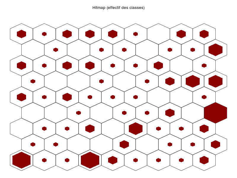
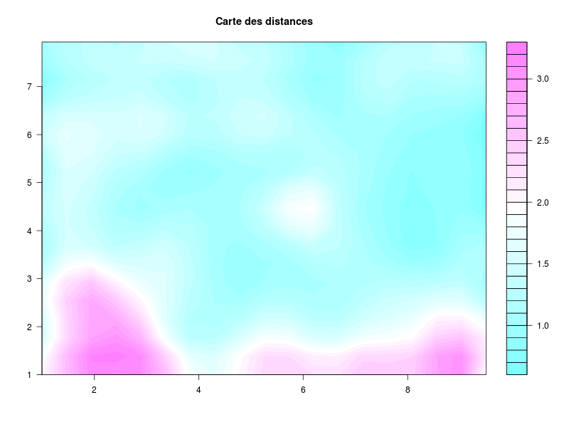
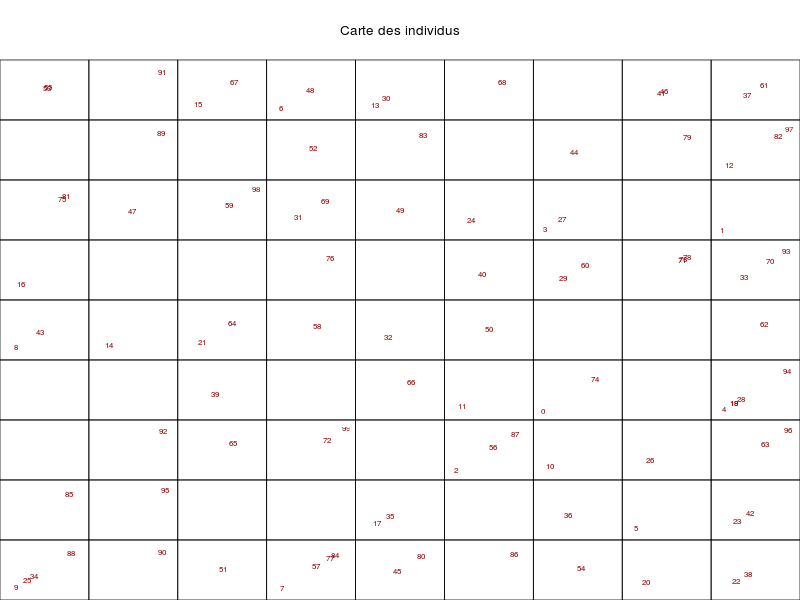
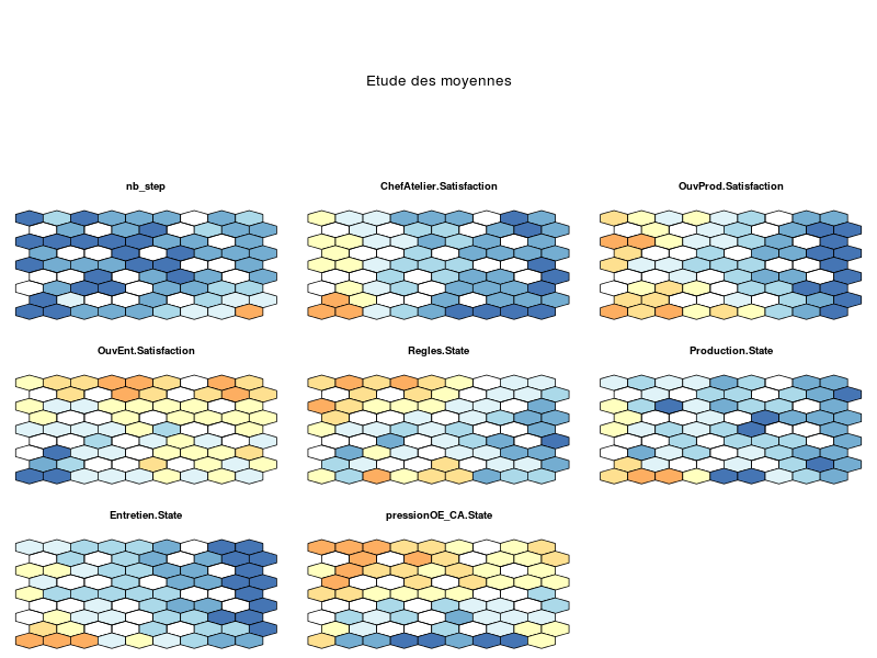
that are automatically saved into the directory from which the data file has been loaded. The function also outputs an object of class som; see:

help(batchsom)

in R for further details on this class.

Download

Pre-requisites

the free statistical software environment R which is available for Windows, Mac and Linux. Mac users must also install additional tools including tcltk;
additional packages:
- ellipse (for plotting ellipses);
- aplpack (for plotting bagplots);
- RColorBrewer (for color palettes);
- xtable (for table exportations in LaTeX and HTML formats);
- yasomi (for self-organizing maps). Warning! This package is still in beta version and is thus not available on CRAN repositories. More information on how to install yasomi at this link. yasomi depends on e1071 and on proxy.

SocLab scripts download

The scripts can be downloaded as a ZIP archive. The dependencies between the functions are displayed in the foodweb image below:

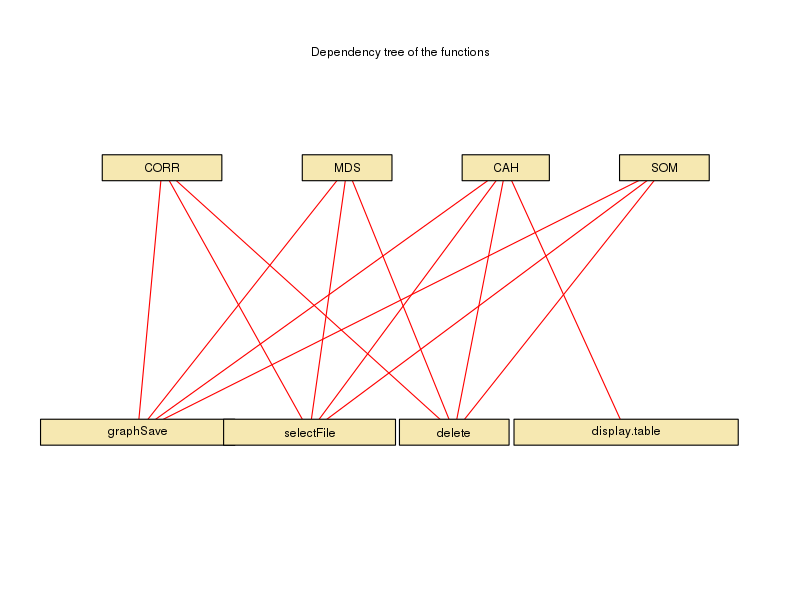
an example data set simulation-Seita.csv with a PDF file In French briefly describing it (see also (Crozier, 1964) in the References section)
a user manual In French written by Soraya Popic which lists all options and provides several examples on how to use the scripts with the data set simulation-Seita.csv.

Using the scripts

unzip the archive containing the scripts in R working directory;
source all scripts. This can be performed with:

files <- list.files(pattern=".[.]R")
sapply(files,source)

use one of the command lines described above, select the file you want to proceed and… voilà!

Warning! The dataset on which you want to perform the analyses must have a format close to that presented in the Examples section (text file, the first line contains the variable names, the columns are separated by a given character which can be a comma, a tabulation, …, specified to the function with the option delim).

References

If you are using these scripts, please cite:

N. Villa-Vialaneix, C. Sibertin-Blanc and P. Roggero. Statistical exploratory analysis of agent-based simulations in a social context. Case Studies in Business, Industry and Government Statistics, 5(2), 132-149, 2014.

On SocLab

(Sibertin-Blanc et al, 2013) C. Sibertin-Blanc, P. Roggero, F. Adreit, B. Baldet, P. Chapron, J. El Gemayel, M. Mailliard. SocLab: A Framework for the Modelling, Simulation and Analysis of Power in Social Organizations. Journal of Artificial Societies and Social Simulation, 16(4): 8, 2013.

On the SEITA dataset

(Crozier, 1964) M. Crozier. Le Phénomène Bureaucratique. Le Seuil, Paris, France, collection points et essais edition, 1964.

On statistical methods

Correlation: see Wikipédia page on Pearson correlation coefficient;
Multi-dimensional scaling
- (Kruskal & Wish, 1978) J.B. Kruskal, and M. Wish. Multidimensional Scaling. Sage, 1978.
- (Hastie et al., 2009) T. Hastie, R. Tibshirani, and J. Friedman. Elements of Statistical Learning. Springer-Verlag, 2nd edition, 2009. (MDS : chapitre 14.8)
Bagplot: have look at this page on Arthur Charpentier’s blog
Hierarchical clustering (Hastie et al., 2009) (chapitre 14.3)
Self-organizing maps
- (Kohonen, 2001) T. Kohonen. Self-organizing maps. Springer Series in Information Sciences, Vol. 30, Springer, Berlin, 3rd extended edition, 2001.
- Marie Cottrell’s course In French

On R

Books co-edited by the Presses Universitaires de Rennes (PUR) and the Société Française de Statistique (SFdS):
- (Cornillon et al., 2011) P.A. Cornillon, A. Guyader, F. Husson, N. Jégou, J. Josse, M. Kloareg, E. Matzner-Løber, and L. Rouvière. Statistiques avec R. Presses Universitaires de Rennes, 3ème édition revue et augmentée, 2011.
- (Husson et al., 2009) F. Husson, S. Lê, and J. Pagès. Analyse de données avec R. Presses Universitaires de Rennes, 2009.
- my own blog and in particular this post and that are directly related to Soraya’s internship.